Introduction

Vector search has quickly become a core building block of modern applications, powering semantic search, recommendation systems, similarity matching, and Retrieval-Augmented Generation (RAG) workflows for LLMs. Instead of searching for exact keywords, vector databases enable meaning-based search using embeddings (vector representations of text, images, audio, or other unstructured data) and fast nearest-neighbor retrieval algorithms.

If you’re experimenting with vector search for the first time or you’re building a prototype and want something you can iterate on quickly, you’ll want a lab environment that’s:

• Local with no cloud dependency required.
• Repeatable, easy to spin up, tear down, and rebuild.
• Close to real-world architecture, so what you learn carries forward.

That’s exactly what we’ll build in this post - but before diving in, let’s look at why AIStor and Milvus are a good fit for workloads that require semantic search.

Why AIStor + Milvus?

Milvus is a vector database that includes a variety of algorithms for performing similarity searches on unstructured data vectorized by an embedding model. It is commonly deployed on-premises when the data it stores contains sensitive information that cannot exist in a public cloud. Vector databases require a storage solution to persist embeddings, index files generated from the vectors, segmentation data, and any other data that must be stored alongside the embeddings, such as the text from which the embeddings were created. Milvus uses MinIO AIStor for its storage solution. AIStor provides a high-performance S3-compatible object store that performs just as well on your local machine as in production environments.

What we’re building

In this tutorial, we will set up a complete vector database “lab” using Docker Compose, combining:

• Milvus: the vector database engine for indexing and similarity searches.
• MinIO AIStor Free: S3-compatible object storage layer to persist embeddings, index files generated from the vectors, segmentation data, and any other data.
• etcd: Milvus uses etcd as its metadata and coordination service.

At the end of this post, you’ll have a working environment you can run on a laptop or workstation, plus a simple demo script to insert vectors and run similarity queries—perfect for experimenting with your own embeddings and datasets.

Introducing AIStor Free

In the past, building a laboratory environment like the one we will create here required engineers to use MinIO’s Community Edition for object storage since it did not make sense to purchase AIStor Enterprise for experimentation. Our Community Edition is great for home labs and non-critical workloads; however, for laboratory environments that must create solutions destined for production, there is a better option. AIStor Free is perfect for developers, researchers, and small organizations that are comfortable with a standalone deployment (single instance) but still need all the enterprise capabilities of AIStor Enterprise. We also offer AIStor Enterprise Lite for customers who require a distributed environment and will store less than 400 TB of data. You can read more about our subscription tiers here.

Using AIStor Free is a practical way to explore an enterprise-ready vector database architecture that mirrors how teams build AI data infrastructure today—without needing Kubernetes or a cloud account to get started.

We are now ready to spin up the stack.

Setting up a Laboratory Environment

Before creating containers with Docker Compose, you need to obtain an AIStor Free license key. This takes two minutes - head on over to the AIStor Subscriptions page, click the ‘Getting Started’ button for AIStor Free, enter your name and work email address, and in a few seconds, a license key will be mailed to you.

‍

Next, create the Docker Compose file shown below in your environment. Notice that the license key we just created must be specified in the volumes section of the AIStor service. You can find a copy of the Docker Compose file, along with all other code assets shown in this post, here.

‍

services:
etcd:
  container_name: milvus-etcd
  image: quay.io/coreos/etcd:v3.5.25
  environment:
    - ETCD_AUTO_COMPACTION_MODE=revision
    - ETCD_AUTO_COMPACTION_RETENTION=1000
    - ETCD_QUOTA_BACKEND_BYTES=4294967296
    - ETCD_SNAPSHOT_COUNT=50000
  volumes:
    - ${VOLUME_PATH}/etcd:/etcd
  command: etcd -advertise-client-urls=http://etcd:2379 -listen-client-urls http://0.0.0.0:2379 --data-dir /etcd
  healthcheck:
    test: ["CMD", "etcdctl", "endpoint", "health"]
    interval: 30s
    timeout: 20s
    retries: 3

minio:
  container_name: milvus-aistor
  image: quay.io/minio/aistor/minio
  environment:
    MINIO_ACCESS_KEY: ${MINIO_ACCESS_KEY}
    MINIO_SECRET_KEY: ${MINIO_SECRET_KEY}
  ports:
    - "9001:9001"
    - "9000:9000"
  volumes:
    - ${VOLUME_PATH}/minio:/minio_data
    - ${AISTOR_LICENSE_FILE}:/minio.license
  command: minio server /minio_data --console-address ":9001"
  healthcheck:
    test: ["CMD", "curl", "-f", "http://localhost:9000/minio/health/live"]
    interval: 30s
    timeout: 20s
    retries: 3

standalone:
  container_name: milvus-standalone
  image: milvusdb/milvus:v2.6.7
  command: ["milvus", "run", "standalone"]
  security_opt:
    - seccomp:unconfined
  environment:
    ETCD_ENDPOINTS: etcd:2379
    MINIO_ADDRESS: minio:9000
    MQ_TYPE: woodpecker
  volumes:
    - ${VOLUME_PATH}/milvus:/var/lib/milvus
  healthcheck:
    test: ["CMD", "curl", "-f", "http://localhost:9091/healthz"]
    interval: 30s
    start_period: 90s
    timeout: 20s
    retries: 3
  ports:
    - "19530:19530"
    - "9091:9091"
  depends_on:
    - "etcd"
    - "minio"

networks:
default:
  name: milvus

‍

To start it, use the command below. Note that I am using a config.env file to specify the AIStor Free license key, usernames, passwords, and the volume drive location.

‍

docker compose -f docker-compose-cpu.yml --env-file config.env up -d

‍

We now have a fully functional RAG Lab. In the code download for this post, this file is named docker-compose-cpu. 

Let’s give our lab a test by inserting a handful of vectors into Milvus. Once this is done, we can submit a query vector to Milvus and ask it to compute the Euclidean distance between the query vector and the inserted vectors. Ordinarily, the vectors we insert are generated by passing a chunk of text through an embedding model, and the query vector is generated from a user question that is also passed through the same embedding model. However, since I want to keep the number of moving parts in this demo simple, I will create the vectors myself. 

Testing the Vector Database

The code in this section is in the setup_test.ipynb Jupyter notebook in the code download. You will need to run the notebook in an environment where you have installed the pymilvus library, as shown below.

‍

pip install pymilvus

‍

Set up imports and constants

The first step is to set up all needed imports and constants. This is shown below. Milvus runs on port 19530 (because that is what we specified in our Docker Compose file). Also, notice that we are using very small vectors (dimension of 2), which will allow us to double-check Milvus’ math with minimal calculations.

‍

import random
from pymilvus import (
  connections, FieldSchema, CollectionSchema, DataType,
  Collection, utility
)

HOST = "localhost"
PORT = "19530"

COLLECTION_NAME = "demo_vectors"
DIM = 2 #128
TOPK = 5

‍

Create a Collection

Next, we will create a collection. A collection in Milvus is a way to organize like vectors. You can think of it like a table in a relational database.

‍

# Connect to Milvus
connections.connect(alias="default", host=HOST, port=PORT)

# Drop collection if it exists (lab-friendly)
if utility.has_collection(COLLECTION_NAME):
  Collection(COLLECTION_NAME).drop()

# Define schema
pk = FieldSchema(name="id", dtype=DataType.INT64, is_primary=True, auto_id=False)
vec = FieldSchema(name="embedding", dtype=DataType.FLOAT_VECTOR, dim=DIM)
txt = FieldSchema(name="text", dtype=DataType.VARCHAR, max_length=512)

schema = CollectionSchema(
  fields=[pk, vec, txt],
  description="Simple demo collection for vector search"
)

# Create collection
col = Collection(name=COLLECTION_NAME, schema=schema)

‍

Create an Index

We need an index within our collection. We will do this now. IVF_FLAT (Inverted File FLAT) compares vector distances using a two-step approximate nearest neighbor (ANN) search that balances speed and accuracy by avoiding a full scan of the entire dataset. L2 stands for the L2 Euclidean distance, which is the metric used to compare vectors. I will describe this metric further once we are ready to run a query.

‍

# Create an index (IVF_FLAT is a friendly starter index)
index_params = {
  "index_type": "IVF_FLAT",
  "metric_type": "L2",
  "params": {"nlist": 128},
}
col.create_index(field_name="embedding", index_params=index_params)

‍

Insert a handful of vectors

We are now ready to insert some vectors. This is shown below. Notice that what we send to the collection aligns with the schema we created earlier.

‍

# Insert some data
vector_count = 5 #200
ids = list(range(1, vector_count + 1))

vectors = []
vectors.append([0,1])
vectors.append([0,2])
vectors.append([0,3])
vectors.append([0,-1])
vectors.append([0,5])
#vectors = [make_vector(DIM) for _ in range(vector_count)]

# Create sample text for each vector.
texts = [f'sample item {i}' for i in ids]

col.insert([ids, vectors, texts])
col.flush()

‍

Load the collection and search

Finally, we can query our vector database. Notice that the query matches an exact vector we previously inserted. So we should expect a hit with a distance of zero.

# Load collection for search
col.load()

# Query vector (in a real app: embedding from a model)
#q = [make_vector(DIM)]
q = [[0,1]]

search_params = {"params": {"nprobe": 16}}
results = col.search(
  data=q,
  anns_field="embedding",
  param=search_params,
  limit=TOPK,
  output_fields=["text"],
)

print(f"\nTop {TOPK} results:")
for i, hit in enumerate(results[0], start=1):
  print(f"{i}. id={hit.id}  distance={hit.distance:.4f}  text={hit.entity.get('text')}")

# Optional: verify MinIO usage by checking bucket objects in MinIO Console.
connections.disconnect("default")

‍

The query above produces the following output. As expected we can see that the top hit as a distance of zero.

‍

Top 5 results:

1. id=1  distance=0.0000  text=sample item 1

2. id=2  distance=1.0000  text=sample item 2

3. id=3  distance=4.0000  text=sample item 3

4. id=4  distance=4.0000  text=sample item 4

5. id=5  distance=16.0000  text=sample item 5

‍

Double-checking the results

For fun, let’s do some more checking by hand-calculating a few distances between the query and the entries in the vector database. This will require a little math but it is not complicated. The index we used in our collection uses the L2 Euclidean distance. The standard mathematical formula for calculating the L2 Euclidean distance between two n-dimensional vectors a and b is:

‍

‍

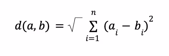
In words, this is the square root of the sum of the squared differences between corresponding components of two vectors. However, to maximize search speed and throughput, Milvus skips the final square root operation and returns the Squared Euclidean Distance. So our equation is reduced to:

‍

This may seem like a bad thing to do but it is OK for the following two reasons:

• Ranking Consistency: The square root does not change the relative rank order of vectors—if a is closer to the query than b in squared distance, it remains closer after the square root is applied.

• Performance: Skipping the square root saves precious compute cycles and lowers latency during searches against large vector databases.

This formula is easier to understand with a concrete example. Let’s calculate the distance between our query and the vector that was an exact match.

‍

(0-0)²+ (1-1)² = 0

‍

Now let’s calculate the distance between the query and the vector that was farthest away.

‍

(0-0)²+ (1-5)² = 16

‍

Both calculations verify the output of our demo script.

Wrap Up

At this point, we built a complete local vector database lab that mirrors how modern AI data stacks are commonly deployed.

Using Docker Compose, we spun up:

• Milvus to handle vector indexing and similarity search.
• MinIO AIStor to persist embeddings, index files generated from the vectors, segmentation data, and any other data.
• etcd as a service to manage metadata, coordination, and internal data flow.

We also verified our lab with an end-to-end demo, inserting vectors and running a similarity query—proving that the stack isn’t just running, but actually capable of useful work.

Next Steps

From here, you can extend this lab in several directions:

• Build a RAG pipeline by plugging in a real embedding model and an open-source LLM.
• Performance-tune the RAG pipeline by loading your own domain-specific dataset and exploring index types and chunking strategies.
• Experiment with Milvus’ GPU capabilities. It is possible to run indexing and semantic searches on a GPU, greatly improving performance. The code download for this post includes a Docker Compose file that uses a GPU-capable Milvus image.
• Experiment with multi-node Milvus or Kubernetes deployments.  For this, you will need AIStor Enterprise Lite or AIStor Enterprise.
• Use this lab as the basis for creating more complex demos, workshops, and internal training.

If you’re evaluating vector databases or designing AI infrastructure, having a hands-on environment like this is invaluable. You can iterate quickly, observe how data flows through the system, and build confidence before moving to more complex deployments.

‍